part04분류-1
분류는 종속변수가 범주형인 방법론이다.
종속변수가 범주형이라는 측면에서 회귀와 대비됨
로지스틱 회귀(logistic regreesion)
-종속변수를 0과 1 사이로 산출하게 하는 로지스틱 함수(시그모이드 함수)를 이용
-ln(p(x)/(1-p(x)) = B0+B1*X
-오즈=성공확률/실패확률
import numpy as np
import pandas as pd
import statsmodels.api as sm
from sklearn.preprocessing import LabelEncoder
from matplotlib import pyplot as plt
import seaborn as sns
import missingno as msno
%matplotlib inline
import warnings
warnings.filterwarnings('ignore')
train=pd.read_csv('data/classification/train.csv')
test=pd.read_csv('data/classification/test.csv')
gender=pd.read_csv('data/classification/gender_submission.csv')
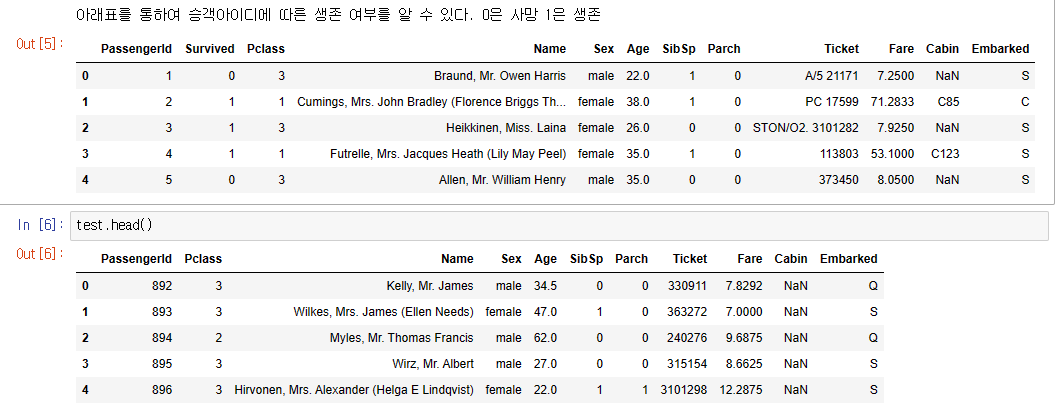
print("아래표를 통하여 승객아이디에 따른 생존 여부를 알 수 있다. 0은 사망 1은 생존")
train.head()
print("test셋에는 생존칼럼이 있지 않으니 생존 칼럼을 추가한다.")test['Survived']=gender['Survived']df=pd.concat([train,test])df.columns.tolist()test셋에는 생존칼럼이 있지 않으니 생존 칼럼을 추가한다.
['PassengerId',
'Survived',
'Pclass',
'Name',
'Sex',
'Age',
'SibSp',
'Parch',
'Ticket',
'Fare',
'Cabin',
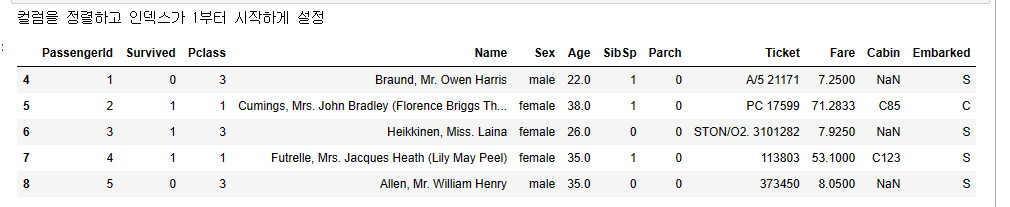
'Embarked'print("컬럼을 정렬하고 인덱스가 1부터 시작하게 설정")
df = df[['PassengerId',
'Survived',
'Pclass',
'Name',
'Sex',
'Age',
'SibSp',
'Parch',
'Ticket',
'Fare',
'Cabin',
'Embarked']]
# index reset
df.reset_index(drop=True)
df.reset_index()
# index를 1부터 시작
df.index += 1
df.head()
print("결측치가 존재하는지 확인. missingno모듈 사용하면 결측치가 있는지 시각적으로 알 수 있다.")
msno.matrix(df,figsize=(16,8))
결측치가 존재하는지 확인. missingno모듈 사용하면 결측치가 있는지 시각적으로 알 수 있다.
<AxesSubplot: >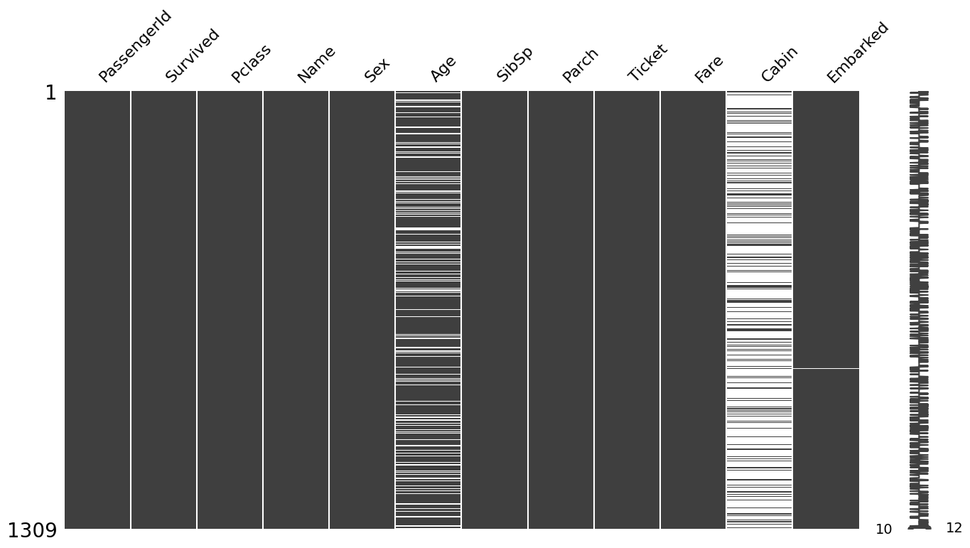
print("결측치를 간단한 숫자로 확인")df.isnull().sum()결측치를 간단한 숫자로 확인
PassengerId       0
Survived          0
Pclass            0
Name              0
Sex               0
Age             263
SibSp             0
Parch             0
Ticket            0
Fare              1
Cabin          1014
Embarked          2
dtype: int64
print("분류를 쉽게 하기 위해서 null이 포함된 row들을 제거, cabin은 null이 많으니 컬럼자체를 제거")df_titanic=df.drop(['Cabin'],axis=1)df_titanic=df_titanic.dropna()df_titanic.isnull().sum()분류를 쉽게 하기 위해서 null이 포함된 row들을 제거, cabin은 null이 많으니 컬럼자체를 제거
PassengerId    0
Survived       0
Pclass         0
Name           0
Sex            0
Age            0
SibSp          0
Parch          0
Ticket         0
Fare           0
Embarked       0
dtype: int6
df_stats = df_titanic.describe().T
skew_results = []
kurtosis_results = []
null_results = []
median_results = []
for idx, val in enumerate(df_stats.index):
median_results.append(df_titanic[val].median())
skew_results.append(df_titanic[val].skew())
kurtosis_results.append(df_titanic[val].kurtosis())
null_results.append(df_titanic[val].isnull().sum())
df_stats['median'] = median_results
df_stats['missing'] = null_results
df_stats['skewness'] = skew_results
df_stats['kurtosis'] = kurtosis_results
print("아래표를 보면 Fare의 값이 4.12로 왼쪽으로 치우쳐져 있다")
df_stats

print("히스토그램으로 다시 Fare을 살펴본다.")
df_titanic['Fare'].hist()
히스토그램으로 다시 Fare을 살펴본다.
<AxesSubplot: >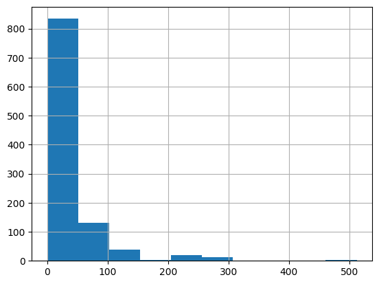
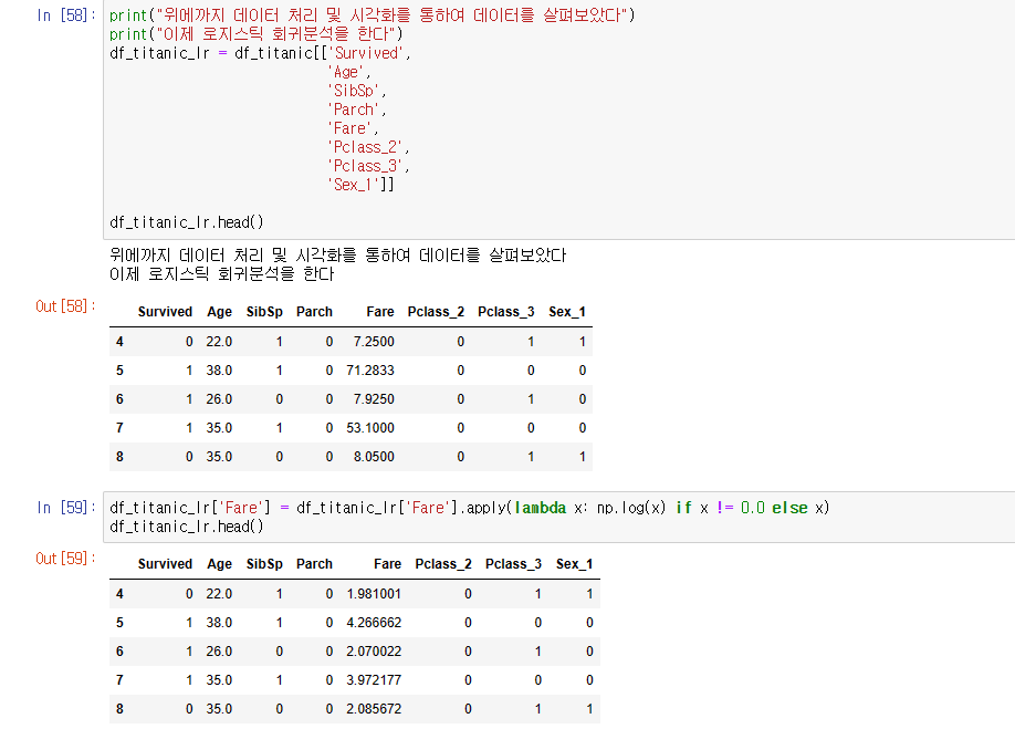
print("Fare값은 로지스틱 분석 전에 자연로그값을 이용하여 고르게 분포하도록 작업한다")
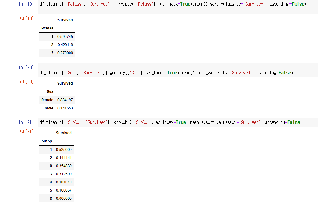
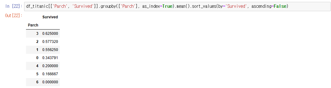
print("아래 표들을 통하여 좌석등급이 높을 수록, 성별은 여성, sibsp수는 1명 , 부모와 자식수는 3인경우가 생존율이 높았다")
total = df_titanic['Survived'].value_counts()[0] + df_titanic['Survived'].value_counts()[1]
print("Survied = 0 은 ", round(df_titanic['Survived'].value_counts()[0] / total *100, 2), '퍼센트')
print("Survied = 1 은 ", round(df_titanic['Survived'].value_counts()[1] / total *100, 2), '퍼센트')
Survied = 0 은 60.21 퍼센트
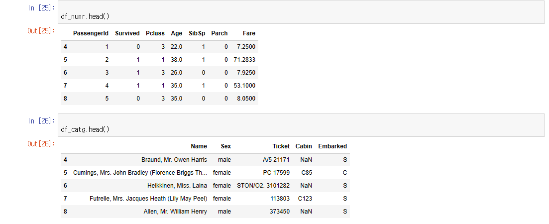
Survied = 1 은 39.79 퍼센트def separate_dtype(df):
df_catg = df.select_dtypes(include=['object'])
df_numr = df.select_dtypes(include=['int64', 'float64'])
return [df_catg, df_numr]
(df_catg, df_numr) = separate_dtype(df)
print("수치형 데이터와 범주형+오브젝트형 타입으로 나눈다")
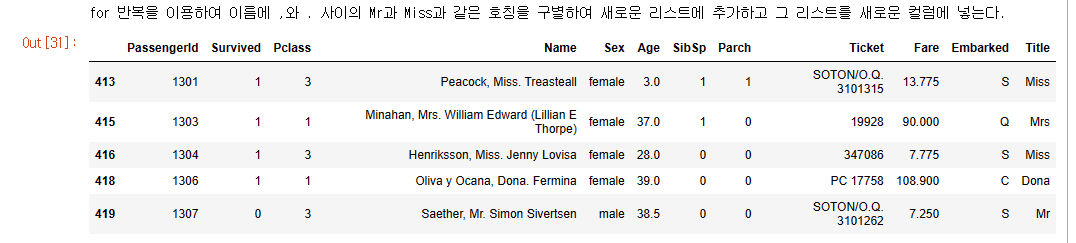
print("for 반복을 이용하여 이름에 ,와 . 사이의 Mr과 Miss과 같은 호칭을 구별하여 새로운 리스트에 추가하고 그 리스트를 새로운 컬럼에 넣는다.")
arr_title = list()
for s in df_titanic['Name'].values:
title = s.split(",")[1].split(".")[0].replace(" ", "")
arr_title.append(title)
df_titanic['Title'] = arr_title
df_titanic.tail()
df_titanic['Title'].value_counts()
Mr             580
Miss           209
Mrs            169
Master          53
Rev              8
Dr               7
Col              4
Mlle             2
Major            2
Ms               1
Lady             1
Sir              1
Mme              1
Don              1
Capt             1
theCountess      1
Jonkheer         1
Dona             1
Name: Title, dtype: int6
print("Mr, Miss, Mrs, Master를 제외하고 이외의 것들은 Others로 분류한다.")
df_titanic['Title'] = df_titanic['Title'].replace(['Rev','Dr','Col','Major','Sir','Don','Lady','theCountess'
,'Jonkheer','Dona','Capt'],'Others')
df_titanic['Title'] = df_titanic['Title'].replace('Mlle','Miss')
df_titanic['Title'] = df_titanic['Title'].replace('Ms','Miss')
df_titanic['Title'] = df_titanic['Title'].replace('Mme','Mrs')
df_titanic['Title'].value_counts()
Mr, Miss, Mrs, Master를 제외하고 이외의 것들은 Others로 분류한다.
Mr        580
Miss      212
Mrs       170
Master     53
Others     28
Name: Title, dtype: int64
df_titanic['Sex'].value_counts()
male      657
female    386
Name: Sex, dtype: int6
print("사이킷런을 이용하요 성별은 여자는0 남자는 1로 처리한다")
enc = LabelEncoder()
enc.fit(df_titanic['Sex'])
df_titanic['Sex'] = enc.transform(df_titanic['Sex'])
df_titanic['Sex']
사이킷런을 이용하요 성별은 여자는0 남자는 1로 처리한다
4      1
5      0
6      0
7      0
8      1
      ..
413    0
415    0
416    0
418    0
419    1
Name: Sex, Length: 1043, dtype: int32
print("정박항구인 Embarked는 S,C,Q로 분류 되어있으며 이것도 각각 0,1,2로 처리")
df_titanic['Embarked'].value_counts()
정박항구인 Embarked는 S,C,Q로 분류 되어있으며 이것도 각각 0,1,2로 처리
S    781
C    212
Q     50
Name: Embarked, dtype: int64
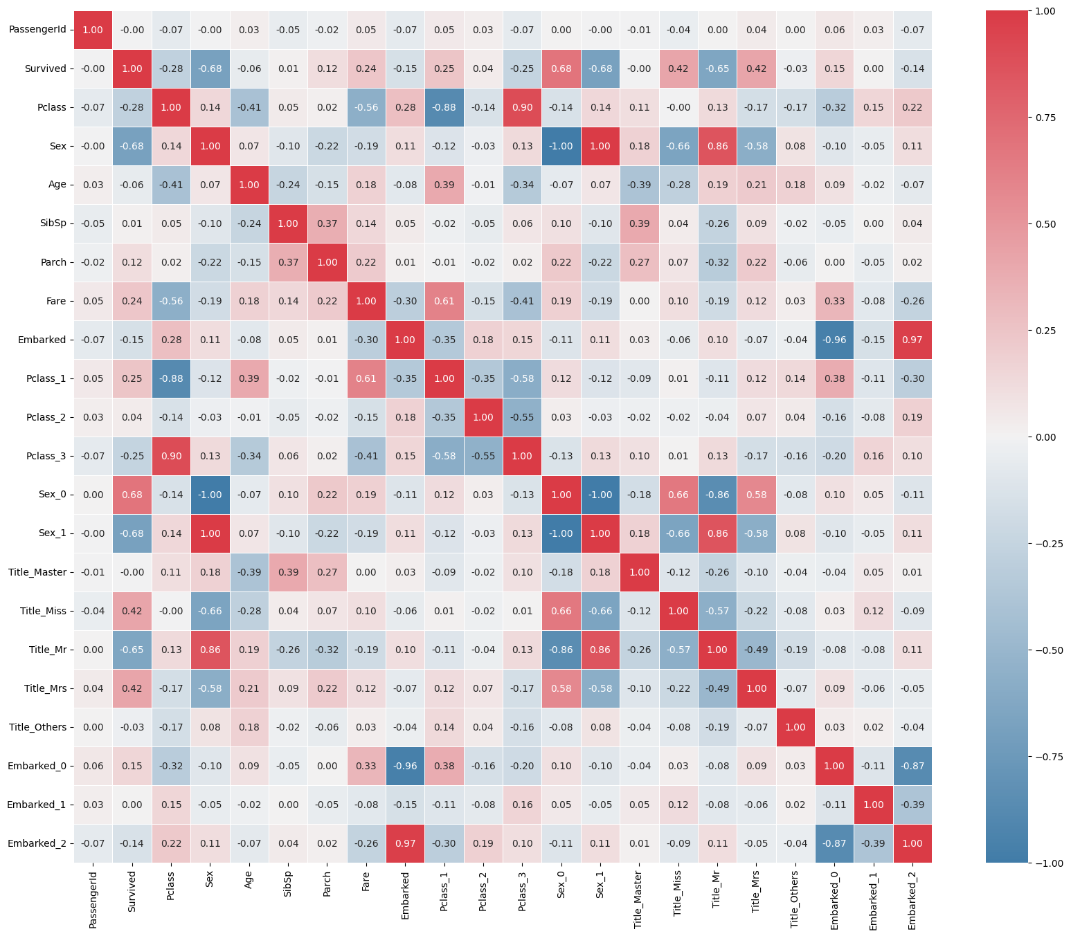
cmap = sns.diverging_palette(240, 10, n=9, as_cmap=True)
plt.figure(figsize=(20,16))
sns.heatmap(df_titanic.corr(), annot=True, cmap = cmap, linewidths=.5, fmt = '.2f', annot_kws={"size":10})
plt.show()
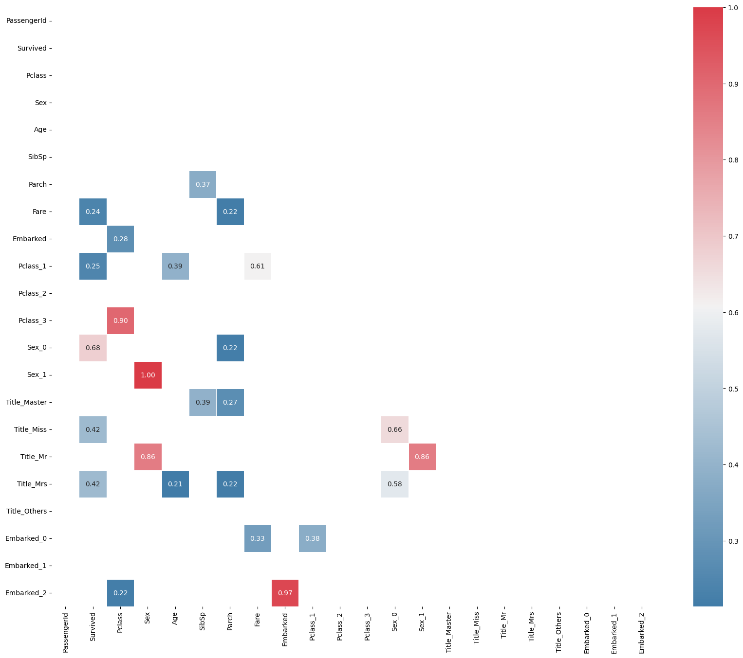
df_corr = df_titanic.corr()
mask = np.zeros_like(df_corr, dtype=np.bool)
mask[np.triu_indices_from(mask)] = True
df_corr_positive = df_corr[df_corr >= 0.2]
df_corr_negative = df_corr[(df_corr <= -0.2) & (df_corr <= 0.99) | (df_corr == -1.0)]
plt.figure(figsize=(20,16))
sns.heatmap(df_corr_positive, annot=True, mask=mask, cmap=cmap, linewidths=.6, fmt = '.2f', annot_kws={"size":10})
plt.show()

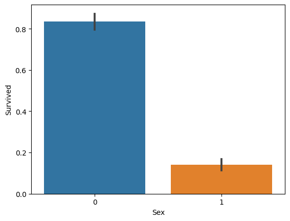
print("종속변수 생존과 성별간의 상간관계를 알아본다.")
sns.barplot(x='Sex', y='Survived', data=df_titanic)
sns.barplot(x='Title', y='Survived', data=df_titanic)

sns.barplot(x='Pclass', y='Survived', data=df_titanic)
<AxesSubplot: xlabel='Pclass', ylabel='Survived'>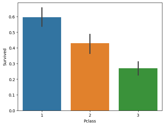
sns.barplot(x='Sex',y='Survived', hue='Title', data=df_titanic)
<AxesSubplot: xlabel='Sex', ylabel='Survived'>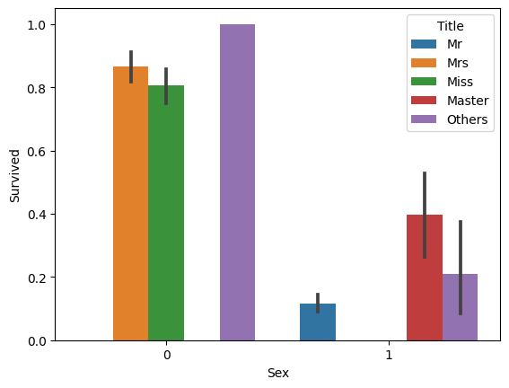
sns.barplot(x='Pclass',y='Survived', hue='Sex', data=df_titanic)

df_titanic_lr['Fare'].hist()
